Vector Algorithm
Algorithm Overview
The algorithm detects regions with abnormal market activity — moments when price ranges increase sharply over a short period. The algorithm allows users to quickly enter such movements and capture profits on short-term market impulses.
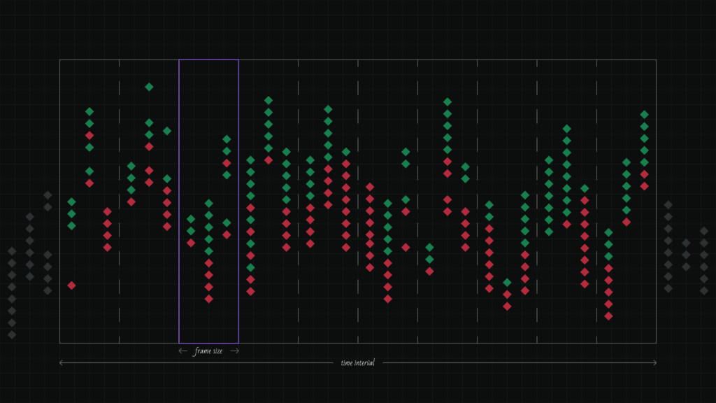
The algorithm analyzes the market in small time intervals (frames), tracks price changes and trading activity, and then automatically places orders when specified conditions are met.
How the Algorithm Works
Operating Principle
- Time Division into Frames The time interval (Time Frame) is divided into small segments — frames (Frame Size). For example, if Time Frame = 2 seconds and Frame Size = 0.2 seconds, the algorithm needs 10 frames for analysis.
- Data Collection in Each Frame In each frame, the algorithm analyzes:
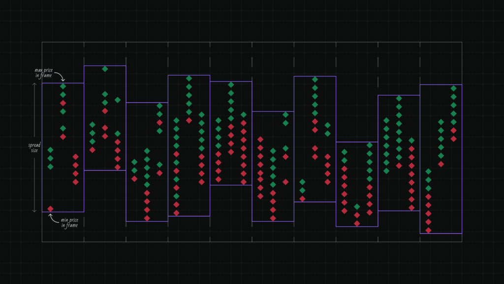
- minimum and maximum trade prices in the frame;
- number of trades;
- trade volumes.
- Entry Condition Check The algorithm generates an entry signal if:
- the spread size (difference between maximum and minimum price) in each frame exceeds the specified percentage (Min Spread Size);
- the direction of movement of the upper and lower spread boundaries corresponds to the specified ranges (Upper/Lower Border Range) (if enabled);
- the number of trades in each frame exceeds the minimum value (Min Trades Per Frame);
- the trading volume in each frame exceeds the minimum (Min Quote Asset Volume).
- Order Placement When the trigger activates, the algorithm places orders:
- for buy: at Order Distance from the lower spread boundary;
- for sell: at Order Distance from the upper spread boundary;
- with the frequency specified by the Order Frequency parameter;
- until Max Orders is reached.
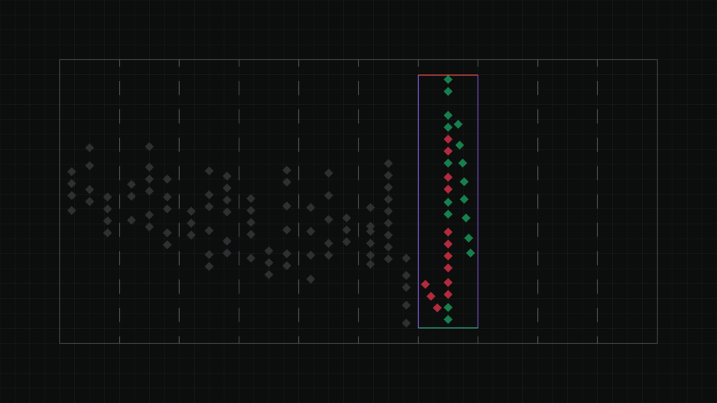
- Position Management After order execution, Take Profit is activated:
- for buy: calculated from the lower spread boundary of the current (latest) frame;
- for sell: calculated from the upper spread boundary of the current (latest) frame.
- The Take Profit value is specified as a percentage of the spread size, not as a percentage of price
Algorithm Configuration
Main Parameters

1. Frame Size
The size of the micro-interval in seconds into which the Time Frame is divided.
The smaller the Frame Size, the more precise the analysis, but the higher the data frequency requirements. This is one of the two key parameters defining the algorithm’s principle.
Default value: 0.2 seconds
Minimum value: 0.001 seconds
Maximum value: unlimited
2. Time Frame
The duration of the time window for analysis in seconds.
This is the total period over which the algorithm analyzes market activity. This is the second key parameter defining the algorithm’s principle. Setting very short intervals — the algorithm will look for only spikes that repeat as frequently as the Time Frame is divided. Setting longer intervals — the algorithm will look for markets that remain in a state of volatility throughout the specified time.
Default value: 1 second
Minimum value: 0.001 seconds
Maximum value: unlimited
3. Min Spread Size
The minimum price range size as a percentage.
The spread is the difference between the maximum and minimum price in a frame. The algorithm generates a signal only if the spread in each frame exceeds the specified value.
Default value: 0.5%
Minimum value: 0%
Maximum value: unlimited
4. Upper Border Range

The filter tracks how the upper spread boundary changes from frame to frame.
The algorithm measures the change in the upper boundary between adjacent frames as a percentage of the last frame’s spread. Specify the minimum and maximum range values. All changes must fall within the specified range — if at least one falls out of range, the condition is not met.
How it works:
Change = (Upper boundary of next frame — Upper boundary of previous frame) / Last frame spread × 100%
Example: 4 frames with upper boundaries 100, 101, 102, 105. Last frame spread = 5.
Changes: (101-100)/5 × 100 = +20%, (102-101)/5 × 100 = +20%, (105-102)/5 × 100 = +60%
Range from +10% to +70% → all changes fit ✅
Range from +10% to +50% → last change (+60%) is out of bounds ❌
Range values:
- Positive values — upper boundary is rising (price moving up)
- Negative values — upper boundary is falling (price moving down)
- Range allows filtering movement strength
Use the checkbox to enable or disable the filter.
Usage: combine with Lower Border Range to find unidirectional movements. For example, for an uptrend, set positive values for both boundaries.
Default value: from 0% to 0.5%
Minimum value: unlimited
Maximum value: unlimited
5. Lower Border Range
The filter tracks how the lower spread boundary changes from frame to frame.
The algorithm measures the change in the lower boundary between adjacent frames as a percentage of the last frame’s spread. Specify the minimum and maximum range values. All changes must fall within the specified range — if at least one falls outside, the condition is not met.
How it works:
Change = (Lower boundary of next frame — Lower boundary of previous frame) / Last frame spread × 100%
Example: 4 frames with lower boundaries 50, 51, 52, 53. Last frame spread = 3.
Changes: (51-50)/3 × 100 = +33.3%, (52-51)/3 × 100 = +33.3%, (53-52)/3 × 100 = +33.3%
Range from +20% to +40% → all changes fit ✅
Range from +20% to +30% → all changes (+33.3%) are out of bounds ❌
Range values:
- Positive values — lower boundary is rising (price moving up)
- Negative values — lower boundary is falling (price moving down)
- Range allows filtering movement strength
Use the checkbox to enable or disable the filter.
Usage: combine with Upper Border Range to find unidirectional movements. For example, for an uptrend, set positive values for both boundaries.
Default value: from 0% to 0.5%
Minimum value: unlimited
Maximum value: unlimited
6. Min Trades Per Frame
The minimum number of trades that must occur in each frame.
This parameter filters low-activity periods. If there are fewer trades in a frame than the specified value, the frame is not considered.
Default value: 2
Minimum value: 0
Maximum value: unlimited
7. Min Quote Asset Volume
The minimum trading volume in the quote currency for each frame.
Helps avoid entering the market during low liquidity. If the trade volume in a frame is less than the specified value, the frame is not considered.
Default value: 10,000
Minimum value: 0
Maximum value: unlimited
8. Order Distance
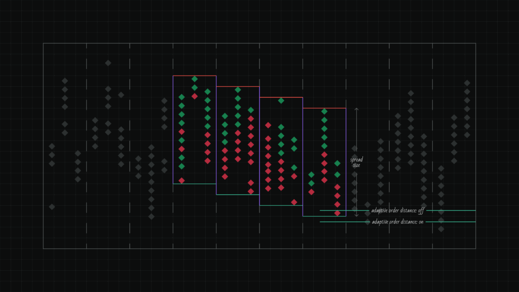
The distance as a percentage of the spread size at which the order will be placed relative to the boundary.
How it works:
Order Distance is calculated as a percentage of the spread size (difference between upper and lower boundaries).
- For Buy: the order is placed above the lower boundary by the specified percentage of the spread
- For Sell: the order is placed below the upper boundary by the specified percentage of the spread
Example for Buy:
Lower boundary = 70
Spread = 5
Order Distance = 5%
Distance in points = 5 × 5% = 0.25
Order price = 70 + 0.25 = 70.25
The larger the Order Distance value, the farther the order is from the boundary and closer to the opposite side of the spread. Negative values place the order outside the spread (below the lower boundary for Buy or above the upper boundary for Sell).
Default value: 5%
Minimum value: unlimited (negative values accepted)
Maximum value: unlimited (values above 100% accepted)
9. Use Adaptive Order Distance
The algorithm automatically adjusts Order Distance taking into account the direction of movement of the spread boundary.
When adaptation is enabled, the algorithm analyzes how the corresponding spread boundary changed between all frames in the Time Frame, calculates the average change, and adds it to the base order price. This allows placing orders more aggressively in the direction of the trend.
How it works:
- The algorithm counts the boundary change between each pair of adjacent frames
- Calculates the average change in absolute price units
- Adds this value to the base order price
Average change formula:
((a2-a1) + (a3-a2) + (a4-a3) + …) / n
where a — boundary value in each frame, n — number of transitions between frames.
For Buy: lower spread boundary is used
For Sell: upper spread boundary is used
Example for Buy:
4 frames with lower boundaries: 76, 74, 72, 70
Last frame: lower boundary = 70, spread = 5
Order Distance = 5%
Changes: (74-76) = -2, (72-74) = -2, (70-72) = -2
Average change = (-2 + -2 + -2) / 3 = -2
Without adaptation:
Order price = 70 + (5 × 5%) = 70 + 0.25 = 70.25
With adaptation:
Order price = 70.25 + (-2) = 68.25
The order is placed lower because the lower boundary is steadily falling. If changes are multidirectional (up and down), the average change may be close to zero, and adaptation has almost no effect on the order price.
10. Order Lifetime
The time in seconds during which the order remains active. The algorithm looks for volatility, places an order hoping to participate in the volatility, and removes it if it doesn’t get filled within the expected time. This parameter makes sense to set in correlation with Frame Size/Timeframe.
If the order is not executed within this time — it is automatically canceled.
Default value: 1 second
Minimum value: 0 seconds
Maximum value: unlimited
11. Max Orders
The total number of unfilled orders and open positions.
The algorithm counts orders and positions together. A new order will not be placed if the sum of active orders and open positions has reached the specified limit.
Default value: 3
Minimum value: 0
Maximum value: unlimited
12. Order Frequency
The frequency of placing new orders (in seconds) when the trigger is active.
Important: this parameter replaces the usual «Delay before restart» parameter, as it performs a similar function — controls the interval between order placements.
Default value: 0.1 seconds
Minimum value: 0 seconds
Maximum value: unlimited
13. Detect Shot
Enable this mode to detect sharp price movements followed by a pullback.
When activated, the algorithm analyzes the last frame and looks for sharp price spikes, expecting a pullback by the specified percentage of the maximum movement.
Important: when Detect Shot mode is enabled, the Time Frame, Upper Border Range, and Lower Border Range parameters are not considered, as the algorithm analyzes only the last frame.
Default pullback value: 80%
Minimum value: 0%
Maximum value: 100%
- 100% — full pullback to the starting point of the movement
- 0% — no pullback
Example: if the price sharply rose from 100 to 101 and then pulled back to 100.2, the pullback was 80% of the movement (price went back by 0.8 out of 1).
14. Shot Direction
Select the direction of movement that the algorithm should detect:
- Up — sharp price rise
- Down — sharp price fall
Profit and Risk Management
Take Profit
The profit-taking level as a percentage of the spread size.
- For Buy: calculated from the lower spread boundary in the current frame
- For Sell: calculated from the upper spread boundary in the current frame
Note: unlike other algorithms, in the Vector algorithm, Take Profit is specified as a percentage of the spread distances, not as a percentage of the asset price. This implementation gives the algorithm more flexibility and the ability to capture more profit when finding large price divergences.
For example, an algorithm with the Spread Size parameter = 0.5 will trigger both with a distance of 1.0% and with a distance of 5.0% between prices in frames. With such a large possible difference, it makes more sense to set Take Profit depending on the situation found.
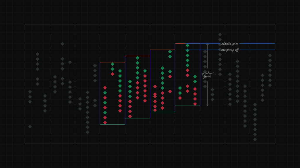
Adaptive Take Profit
The algorithm automatically adjusts the Take Profit distance taking into account the direction of movement of the spread boundary.
When adaptation is enabled, the algorithm analyzes how the corresponding spread boundary changed between all frames in the Time Frame, calculates the average change, and adds it to the base Take Profit price. This allows taking profit with consideration of the current price movement trend.
How it works:
- The algorithm counts the boundary change between each pair of adjacent frames
- Calculates the average change in absolute price units
- Adds this value to the base Take Profit price
Average change formula:
((a2-a1) + (a3-a2) + (a4-a3) + …) / n
where a — boundary value in each frame, n — number of transitions between frames.
For Buy: lower spread boundary is used
For Sell: upper spread boundary is used
Example for Buy:
4 frames with lower boundaries: 100, 110, 120, 130
Last frame: lower boundary = 130, spread = 100
Take Profit = 90%
Changes: (110-100) = +10, (120-110) = +10, (130-120) = +10
Average change = (+10 + +10 + +10) / 3 = +10
Without adaptation:
Take Profit price = 130 + (100 × 90%) = 130 + 90 = 220
With adaptation:
Take Profit price = 220 + (+10) = 230
Take Profit is placed higher because the lower boundary is steadily rising. If changes are multidirectional (up and down), the average change may be close to zero, and adaptation has almost no effect on the Take Profit price.
Stop Loss
The stop-loss level as a percentage of the order placement price.
Contact and Support
If you have questions about algorithm configuration or want to suggest improvements, contact the support team.